Python Programming
Lecture 10 Data Organization and Visualization
10.1 AI辅助编程I:数据整理与清洗

GitHub Copilot官网
尽管 ChatGPT或者Deepseek 可以编写完整的代码,但是要与集成开发环境(Integrated Development Environment,IDE)无缝对按,使用ChatGPT 就不太方便了,尤其是在生成片段代码时,如补全一个函数的定义、补全某个语句等,在这种情况下,使用GitHub Copilot 是一个非常好的选择。当然,最好是将 ChatGPT 与 GitHub Copilot一起使用:使用 ChatGPT 生成一个完整的解决方案,并使用 GitHub Copilot 对这个解决方案进行微调。
- 安装VScode参考配置 参考配置(VScode是什么?常用IDE有哪些?)
- 注册GitHub账户;3. 在VScode里面安装GitHub Copilot插件。

功能介绍
1. 自动补全注释(按Tab键)
# 编写一个程序,读取文件夹中的文件
2. 根据函数名自动生成代码(按Tab键)
def bubblesort()
3. 生成测试用例(在bubblesort函数下方输入)
#测试bubblesort函数
4. 逐步代码生成
#定义5个列表变量,每个列表包含2到10个元素
#将5个列表合并,再调用bubblesort函数对列表排序
5. 自动生成语句架构
for i
-if
6. 生成多个候选解决方案
如果使用Tab键生成解决方案,那么对于一些复杂的代码,可能需要一行一行地生成(需要不断地按 Enter 键和 Tab 键),比较麻烦。GitHub Copilot 提供了生成多个候选解决方案的功能,具体的做法就是在注释中按 Ctrl + Enter 组合键,这将显示一个新的选项卡,默认会自动生成10个解决方案。(有时候还不如直接ChatGPT或者Deepseek)
#用Flask实现一个服务端程序,只支持GET请求,请求的参数是一个字符串,返回一个字符串。
7. 检查代码漏洞
# 检查上面的代码是否有漏洞
一句话就是:写注释,然后enter和tab来回的按。
GitHub Copilot的免费平替CodeGeeX
提示词的编写技巧
- 给AI工具指定一个角色:第一句“你是pandas专家”
- 交代背景:给出文件的路径,以及文件中变量的名称,行列信息
- 说明问题:解决什么问题,必要时说明用什么方法解决,以及指定输出内容,形式和格式
- 必要时给出示例:帮助AI工具理解意图
注意事项
- 提倡用短句,用专用词指定对象,避免使用“它”和“前面”等词
- 明确指定输出内容,可以是全部数据,也可以是一部分
- 指定输出的数据格式,输出文件的路径和名称,甚至编码
10.2 Pandas (3)
Data Organization
Data of Crowdfunding Projects
Kickstarter Projects from Kaggle.com
Loading .csv file
df = pd.read_csv("ks-projects-201801.csv")
relative path
df = pd.read_csv("data/ks-projects-201801.csv") # Linux or OSX
df = pd.read_csv("data\ks-projects-201801.csv") # Windows
absolute path
file_path = '/home/ehmatthes/data/ks-projects-201801.csv'
df = pd.read_csv(file_path) # Linux or OSX

file_path = r'C:\Users\ehmatthes\data\ks-projects-201801.csv'
df = pd.read_csv(file_path) # Windows
Basic Information
>>> df.shape
(378661, 15)

>>> df.info()
RangeIndex: 378661 entries, 0 to 378660
Data columns (total 15 columns):
ID                  378661 non-null int64
name                378657 non-null object
category            378661 non-null object
main_category       378661 non-null object
currency            378661 non-null object
deadline            378661 non-null object
goal                378661 non-null float64
launched            378661 non-null object
pledged             378661 non-null float64
state               378661 non-null object
backers             378661 non-null int64
country             378661 non-null object
usd pledged         374864 non-null float64
usd_pledged_real    378661 non-null float64
usd_goal_real       378661 non-null float64
dtypes: float64(5), int64(2), object(8)
memory usage: 43.3+ MB
Basic Data Description
>>> df_us[['backers','goal','pledged']].describe()
             backers          goal       pledged
count  292627.000000  2.926270e+05  2.926270e+05
mean      113.078615  4.403497e+04  9.670193e+03
std       985.723400  1.108372e+06  9.932942e+04
min         0.000000  1.000000e-02  0.000000e+00
25%         2.000000  2.000000e+03  4.100000e+01
50%        14.000000  5.250000e+03  7.250000e+02
75%        60.000000  1.500000e+04  4.370000e+03
max    219382.000000  1.000000e+08  2.033899e+07
Filtering with boolean array
#根据条件筛选特定行:美国本土项目,筹资金额大于等于30000美刀
>>> df_us = df[df['country']=='US']
>>> df_us30000 = df_us[df_us['goal']>=30000]

#[43312 rows x 15 columns]
Arithmetics
>>> df_us['percentage'] = df_us['pledged']/df_us['goal']
#去掉warning
>>> df_us.copy().loc[:,'percentage'] = df_us['pledged']/df_us['goal']
Sorting and Ranking
When sorting a DataFrame, you can use the data in one or more columns as the sort keys. To do so, pass one or more column names to the by option of sort_values.
>>> df_us.sort_values(by='goal', ascending=False)

>>> df_us.head().sort_values(by=['main_category','goal'],
...: ascending=[True,False])
             ID  ... percentage
2  1.000004e+09  ...   0.004889
1  1.000004e+09  ...   0.080700
4  1.000011e+09  ...   0.065795
5  1.000014e+09  ...   1.047500
3  1.000008e+09  ...   0.000200
>>> df_us.head().rank()
    ID  name  category  ...  usd_pledged_real  usd_goal_real  percentage
1  1.0   2.0       3.5  ...               4.0            3.0         4.0
2  2.0   5.0       3.5  ...               2.0            4.0         2.0
3  3.0   4.0       2.0  ...               1.0            1.0         1.0
4  4.0   1.0       1.0  ...               3.0            2.0         3.0
5  5.0   3.0       5.0  ...               5.0            5.0         5.0
Counting
>>> df_us['main_category'].value_counts()

Film & Video    51922
Music           43238
Publishing      31726
Games           24636
Art             22311
Design          21690
Technology      21556
Food            19941
Fashion         16584
Comics           8910
Theater          8709
Photography      7988
Crafts           6648
Journalism       3540
Dance            3228
Name: main_category, dtype: int64
>>> df_us['main_category'].value_counts(
...: normalize = True)
Film & Video    0.177434
Music           0.147758
Publishing      0.108418
Games           0.084189
Art             0.076244
Design          0.074122
Technology      0.073664
Food            0.068145
Fashion         0.056673
Comics          0.030448
Theater         0.029761
Photography     0.027298
Crafts          0.022718
Journalism      0.012097
Dance           0.011031
Name: main_category, dtype: float64
Time
>>> stamp_0 =pd.to_datetime('2017-09-02 04:43:57')
>>> stamp_0
Timestamp('2017-09-02 04:43:57')
Calculating the time period
>>> df_us['launched_time'] = pd.to_datetime(df_us['launched'])
>>> df_us['deadline_time'] = pd.to_datetime(df_us['deadline'])
>>> df_us['period'] = df_us['deadline_time']-df_us['launched_time']
>>> df_us['period']
1        59 days 19:16:03
2        44 days 23:39:10
3        29 days 20:35:49
4        55 days 15:24:57
5        34 days 10:21:33

378656   29 days 21:24:30
378657   26 days 20:24:46
378658   45 days 04:19:30
378659   30 days 05:46:07
378660   27 days 14:52:13
Name: period, Length: 292627, dtype: timedelta64[ns]
Converting the time to numbers
>>> df_us['period_num'] = df_us['period'].dt.days
>>> df_us['period_num']
1         59.802813
2         44.985532
3         29.858206
4         55.642326
5         34.431632

378656    29.892014
378657    26.850532
378658    45.180208
378659    30.240359
378660    27.619595
Name: period_num, Length: 292627, dtype: float64
Filtering by date
>>> df_us[(df_us['launched_time']>='20150101')]
>>> df_us[(df_us['launched_time']>='20150101')& (df_us['launched_time']<='20151231')]
Summarizing and Computing
>>> df_us.count(axis=1) #每行非空个数
>>> df_us.count(axis=0) #每列非空个数
>>> df_us['usd_pledged_real'].sum()
>>> df_us['usd_pledged_real'].mean()
.max()     .min()
.median()  .mode()
.var()     .std()
.quantile() #0-1
Correlation and Covariance
>>> data = pd.DataFrame({'Q1':[1,3,4,3,4],
...:                     'Q2':[2,3,1,2,3],
...:                     'Q3':[1,5,2,4,4]})
>>> data['Q1'].corr(data['Q3'])
0.4969039949999533

>>> data['Q1'].cov(data['Q3'])
1

>>> data.cov()
>>> data.corr()
Export .csv file
>>> out_col = ['deadline_time','period_num','launched_time']
>>> df_us.to_csv('out.csv',index=False,columns=out_col)
10.2 Pandas (4)
Data Visualization
import pandas as pd
import matplotlib.pyplot as plt
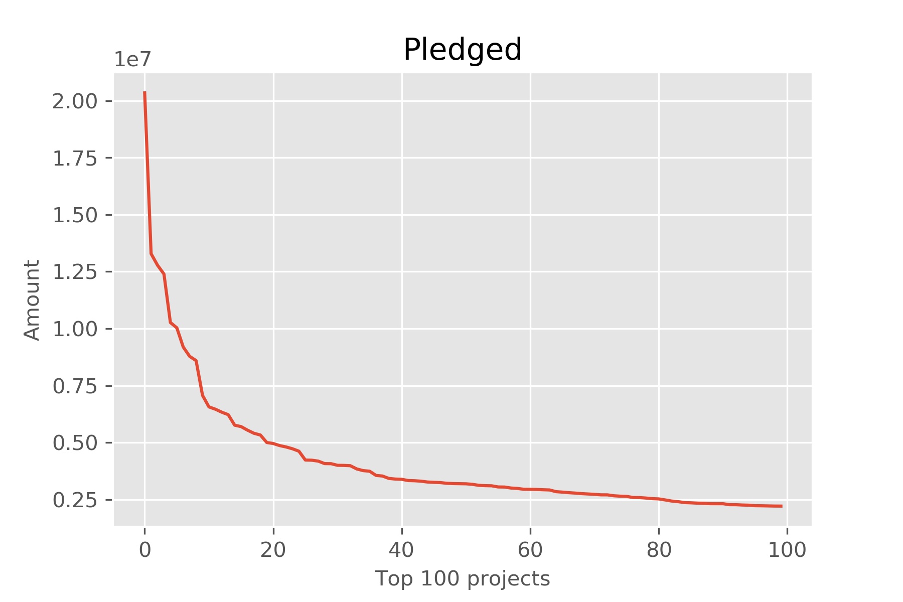
df = pd.read_csv("ks-projects-201801.csv")
df_pledged = df.sort_values(by='pledged',ascending=False).head(100)
fig, ax= plt.subplots()
plt.style.use('ggplot')
ax.plot(df_pledged['pledged'].values)
ax.set_title("Pledged", loc='center')
ax.set_xlabel("Top 100 projects", fontsize=10)
ax.set_ylabel("Amount", fontsize=10)
plt.savefig('pledged.jpg',dpi=300)
Time
import pandas as pd
import matplotlib.pyplot as plt
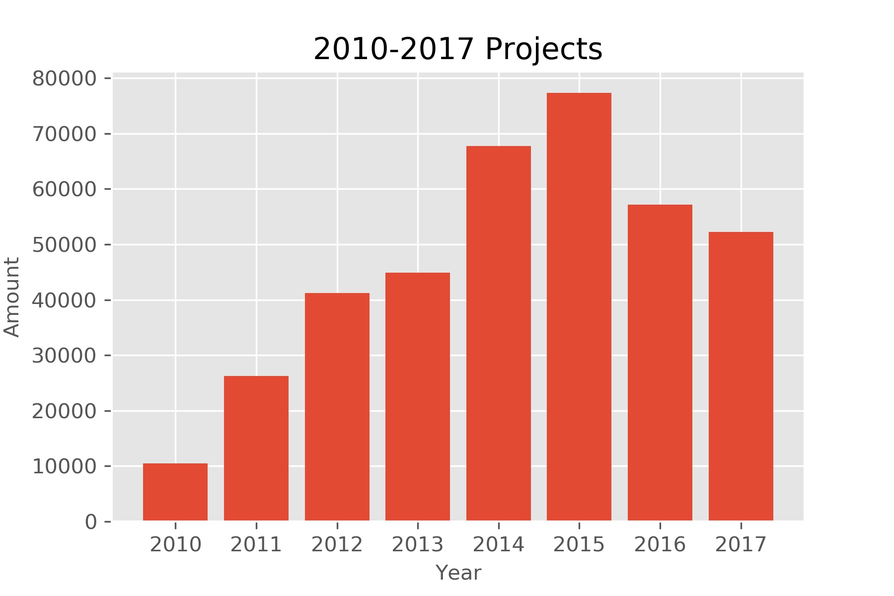
df = pd.read_csv("ks-projects-201801.csv")
df['launched_time'] = pd.to_datetime(df['launched'])
df['deadline_time'] = pd.to_datetime(df['deadline'])
def year_data(y):
    return df[(df['launched_time']>=str(y)) & (df['launched_time']< str(y+1))]

df_year_count=[]
df_year=list(range(2010,2018))
for y in range(2010,2018):
    df_year_count.append(year_data(y)['ID'].count())
fig, ax= plt.subplots()
ax.bar(df_year,df_year_count)
ax.set_title("2010-2017 Projects", loc='center')
ax.set_xlabel("Year", fontsize=10)
ax.set_ylabel("Amount", fontsize=10)
plt.savefig('year.jpg',dpi=300)
Time: Percentage
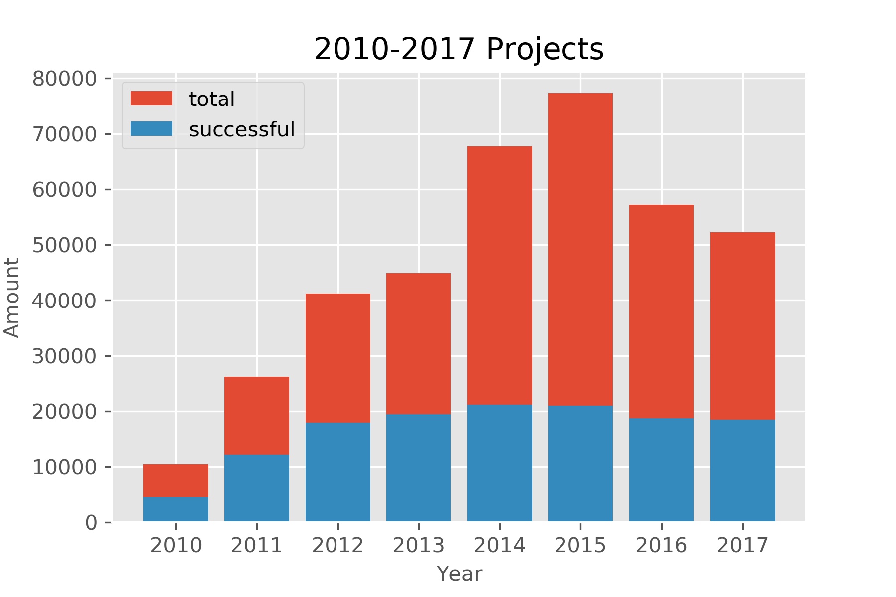
def year_data(y):
    return df[(df['launched_time']>=str(y)) & (df['launched_time']< str(y+1))]

df_year_count=[]
df_year=list(range(2010,2018))
for y in range(2010,2018):
    df_year_count.append(year_data(y)['ID'].count())
df_year_s=[]
for y in range(2010,2018):
    df_year_s.append(year_data(y)[year_data(y)['state']=='successful']['ID'].count())
fig, ax= plt.subplots()
ax.bar(df_year,df_year_count, label='total')
ax.bar(df_year,df_year_s,label='successful')
ax.set_title("2010-2017 Projects", loc='center')
ax.set_xlabel("Year", fontsize=10)
ax.set_ylabel("Amount", fontsize=10)
plt.legend(loc="upper left")
plt.savefig('year_percentage.jpg',dpi=300)
Example
你是pandas专家,文件路径为“/Users/wangwanglulu/ks-projects-201801.csv”。使用pandas导入该文件,根据launched和deadline两列来计算每一个项目的时间跨度,将时间跨度数据作为列添加到原数据中。然后,计算2010年-2018年的项目时间跨度平均值,并绘制横坐标为年份的折线图。最后,保存增加了时间跨度这一列的数据到新的csv文件,并保存图片到jpg文件dpi为300。为代码添加注释。
下载ChatGPT生成的代码Exercise:请根据main_category列,计算每一种类型的百分占比,并绘制柱状图。
数据可视化的系统原则
核心目的:用最少的图形元素传达最多的信息
- 尽量减少多余的装饰元素;
- 信息表达要清晰、准确;
- 避免误导读者对数据的理解。
通用可视化方法论
先问自己:这幅图想回答什么问题?
- 比较(Comparison): 条形图(bar chart):谁大谁小?差多少?
- 趋势(Trend): 折线图(line chart):随时间如何变化?
- 分布(Distribution): 直方图(histogram):集中在哪?有没有极端值?
- 构成(Composition): 堆叠条形图(stacked bar chart):整体由哪些部分组成?占比如何?
- 关系(Relationship): 散点图(scatter plot):两个或多个变量之间的相关性如何?
注意事项
- 避免 3D 图表;
- 饼图能不用就不用,特别是类别大于 3、差异较小或需要精确比较时;
- 颜色不要超过 5 种,且有明确含义;
- 图标题写“结论”,而不是写“图的类型”;
- 不要随意截断 y 轴,防止夸大差异;
- 避免过长、过密的标签,必要时做聚合或缩写;
- 优先使用“小多图”(small multiples)而不是一张拥挤的大图;
- 必要时用文字注释(annotation),帮助读者抓住关键信息。
Summary
- Pandas
- Reading: Python for Data Analysis, Chapter 5, 9, 11.1, 11.2
- Reading: Python for Everybody, Chapter 15.1, 15.2, 16.1